Inia Soto Ramos, From the Mountains of Puerto Rico to Mountains of NASA Earth Data

Name: Dr. Inia Soto Ramos
Title and Formal Job Classification: Associate Research Scientist
Organization: Ocean Ecology Laboratory (Code 616) via Morgan State University and GESTAR II cooperative agreement

What do you do and what is most interesting about your role here at Goddard?

I am currently co-leading the validation efforts for PACE, NASA’s Plankton, Aerosol, Cloud, ocean Ecosystem mission. I am also part of NASA’s SeaBASS (SeaWiFS Bio-optical Archive and Storage System) team, which is responsible for archiving, distributing, and managing field data used for validation and development of satellite ocean color data products. It has been exciting to be a part of a satellite mission, to see it being built, tested and launched. And now, be able to validate the data and in the near future, use the data to do science.

What is your educational background?

I graduated with a bachelor’s degree in biology from The University of Puerto Rico, Mayagüez Campus, and I have a master’s and Ph.D. in Biological Oceanography from the University of South Florida.

How did you get your foot in the door at NASA?

While I was a student at the University of Puerto Rico, I saw a flyer for a program called PaSCoR (Partnership for Spatial and Computational Research). It was a partnership between universities, NASA and other institutions with the intent to train students in remote sensing and Geographical Information Systems. Although, this program was targeted mainly for engineers, I decided to apply. That took me to the first remote sensing classes I had taken. That’s how I started learning that you can study the ocean from space. I had no idea that could be done. That program planted the curiosity about satellite oceanography and gave me the tools to go into graduate school in that field.

How did you first gain exposure to oceanography and diving?

I am from Puerto Rico and grew up all the way in the mountains. There wasn’t much of a connection to the ocean for me, only a few trips to the beach. I remember my dad taking me to a small beach called La Poza del Obispo in Arecibo and he held me while I used a small snorkel underwater. That was the first connection I had with marine life. I started diving sometime when I was about 18 years old, and I remember saying, “This is the most amazing thing ever,” and that’s when I decided I needed to pursue a life in that field.

What interested you in phytoplankton as a specialty?

Initially, I was curious about harmful algal blooms in the West Florida Shelf, which I studied when I moved to Florida to do my grad studies. I learned that the blooms can produce neurotoxins, and those can affect humans in different ways. So, if you have asthma, they can make you feel worse. I remember developing asthma that night after going to the beach and having go to the ER. I didn’t see the connection at the time until I learned about these events and how toxins can get in the air. It felt like something important that I could study to help people or do something that’s meaningful. It’s amazing that we can see something so tiny from space and study them.

How does your identity, being a Latina, show up at NASA?

This is kind of a dream come true. It is so amazing to be able to fulfill that dream. I came from a small town. There appeared to me no chances to come all the way to NASA. So, having this opportunity is exciting, and bringing it back to my community and saying, “Hey, anyone can actually do it.” One of the advantages is that you speak a different language, so you can make connections with different countries.

What do you look forward to in the future? What are some of your goals?

 I would love to keep growing in my field. As a mother, sometimes is hard to visualize where I want to be in the future, so I find it best to focus on the present. My priority right now is my family, however in the future I would love to engage in a job in which I can transfer my knowledge and love to the oceans to future generations; and be more involved in the community.

When you think of your village and growing up in Puerto Rico, what is a memory you have that makes you smile?

I still remember going to collect coffee with my mom and dad. My dad had a small basket for me that I would fill with only the most beautiful red grains of coffee. I was around 5 years old, and I remember the toys that my mom would take, and they’d settle me under the coffee trees. I still go to Puerto Rico, and I am fascinated when I see the coffee trees; it reminds me of my childhood.

What advice would you give to other little girls who might not think NASA is a dream they can achieve?
I was the little girl with the dream of being a scientist at NASA, and then I was a teenager, an adult, and a mother, all with the same dream! It took me several decades and many life stages to get here. Many times, along my path, I thought of giving up. Others, I thought I was completely off track and I would never fulfill my dream. I had limited resources while growing up. There were no fancy swimming or piano classes, but I had amazing teachers and mentors who guided me along the way. So, no matter how young or old you are, you can still fulfill that dream. The key to success is to know where you want to go, surround yourself with people that believe in you, and if you fall, just shake it off and try again!

By Alexa Figueroa
NASA’s Goddard Space Flight Center, Greenbelt, Md.

Conversations With Goddard is a collection of Q&A profiles highlighting the breadth and depth of NASA’s Goddard Space Flight Center’s talented and diverse workforce. The Conversations have been published twice a month on average since May 2011. Read past editions on Goddard’s “Our People” webpage.

Powered by WPeMatico

Get The Details…
Rob Garner

Peculiar Pale Pebbles

During its recent exploration of the crater rim, Perseverance diverted to explore a strange, scattered field of bright white rocks which sparked the interest of the team scientists.

Perseverance has been climbing up the steep slopes of the Jezero crater rim for over two months now, and ever since approaching the edge of the crater has been spying increasingly diverse and strange-looking rocks. Back in the Jezero inlet channel, Neretva Vallis, Perseverance spotted a whole host of colourful boulders at Mount Washburn, and more recently the science team and internet alike were mesmerised by Freya Castle – a rock striped like a zebra! The crater rim hasn’t finished delivering surprises yet though… Just as we humans were preparing for Halloween back on Earth, a ghostly field of bright white rocks appeared in Perseverance’s view, at the base of a mound in the crater rim termed “Mist Park”, and sparking a new mystery for the science team to unravel.

On Earth, we find white rocks in a wide array of geologic settings, and that’s not surprising given the diverse array of light-toned minerals which can be generated across Earth’s various tectonic settings. On Mars however, with its lack of plate tectonics and a basaltic crust dominated by dark minerals like olivine and pyroxene, white rocks are a rare find. The science team planned several observations using Perseverance’s remote sensing instruments to assess the composition of these peculiar pebbles, including multispectral imaging with Mastcam-Z and zapping them with Supercam’s laser. Hopefully these observations can shed light on how these white rocks formed all the way up here on the crater rim. Unfortunately, none of the rocks were big enough to safely inspect them up close with Perseverance’s robotic arm instruments, but the team are on the lookout for larger blocks or outcrops of this strange lithology as we continue traversing upslope.

Aside from their composition, another mystery is just how these rocks got here. The blocks are all float (float = loose rocks, not in their original location), and scattered over just a few square meters. Perhaps these could be erosional leftovers of some kind of resistant vein or rock layer, where the softer, surrounding lithologies have eroded away? Or could these blocks have tumbled downslope from a more continuous bedrock exposure of enigmatic white material? Who knows, but Perseverance will be keeping its eyes peeled for more of these bizarre blocks as it continues to summit new heights…

Written by Alex Jones, PhD student at Imperial College London

Downloads

Perseverance Raw Images

Mars Perseverance Sol 1311: Right Navigation Camera (Navcam)

Nov 12, 2024

PNG ()

Mars Perseverance Sol 1311: Left Mastcam-Z Camera

Nov 12, 2024

PNG ()

Explore More

2 min read

Sols 4359-4361: The Perfect Road Trip Destination For Any Rover!

Article


19 hours ago

4 min read

Sols 4357–4358: Turning West

Article


4 days ago

2 min read

Mars 2020 Perseverance Joins NASA’s Here to Observe Program

The Mars 2020 Perseverance mission has recently joined the NASA Here to Observe (H2O) program,…

Article


6 days ago

Keep Exploring

Discover More Topics From NASA

Mars

Mars is the fourth planet from the Sun, and the seventh largest. It’s the only planet we know of inhabited…

All Mars Resources

Explore this collection of Mars images, videos, resources, PDFs, and toolkits. Discover valuable content designed to inform, educate, and inspire,…

Rover Basics

Each robotic explorer sent to the Red Planet has its own unique capabilities driven by science. Many attributes of a…

Mars Exploration: Science Goals

The key to understanding the past, present or future potential for life on Mars can be found in NASA’s four…

Powered by WPeMatico

Get The Details…

Summary of the Second OMI–TROPOMI Science Team Meeting

Introduction

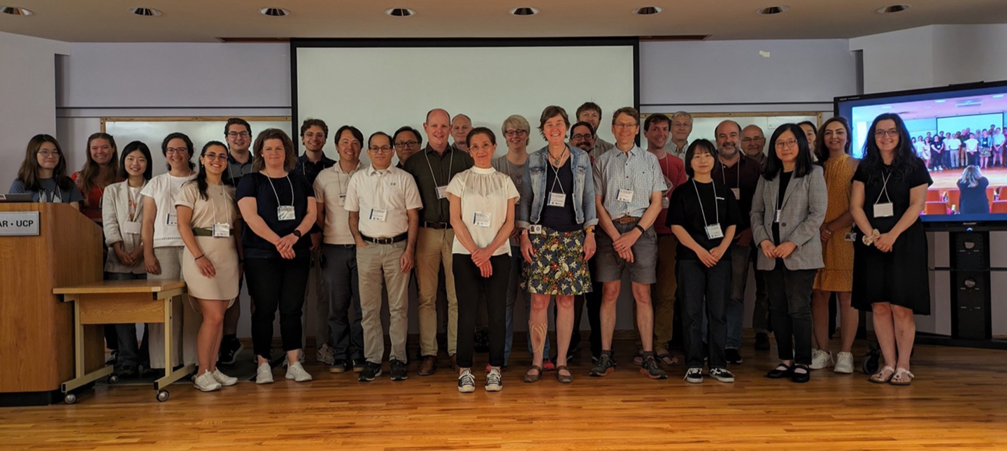
The second joint Ozone Monitoring Instrument (OMI)–TROPOspheric Monitoring Instrument (TROPOMI) Science Team (ST) meeting was held June 3–6, 2024. The meeting used a hybrid format, with the in-person meeting hosted at the National Center for Atmospheric Research (NCAR) in Boulder, CO. This was the first OMI meeting to offer virtual participation since the COVID-19 travel restrictions. Combining the onsite and virtual attendees, the meeting drew 125 participants – see Photo.

OMI flies on NASA’s Earth Observing System (EOS) Aura platform, launched July 15, 2004. TROPOMI flies on the European Space Agency’s (ESA)–Copernicus Sentinel-5 Precursor platform. OMI has collected nearly 20 years of data and TROPOMI now has amassed 5 years of data. 

Meeting content was organized around the following four objectives:

• discussion of the final reprocessing of OMI data (called Collection 4) and of data preservation;
• discussion of OMI data continuity and enhancements using TROPOMI measurements;
• development of unique TROPOMI products [e.g., methane (CH₄)], applications (e.g., tracking emissions – and using them as indicators of socioeconomic and military activities), and new focus regions (e.g., Africa); and
• leverage synergies between atmospheric composition (AC) and greenhouse gas (GHG) missions, which form the international constellation of low Earth orbit (LEO) and geostationary orbit (GEO) satellites.

The remainder of this article summarizes the highlights from each day of the meeting.

DAY ONE

The topics covered on the first day of the meeting included OMI instrument performance, calibration, final Collection 4 reprocessing, and plans for data preservation.

OMI and Data Products Update

Pieternel Levelt [Royal Netherlands Meteorological Institute (KNMI)—OMI Principal Investigator (PI) and NCAR’s Atmospheric Chemistry Observations & Modeling (ACOM) Laboratory—Director] began her presentation by dedicating the meeting to the memory of Johan de Vries, whose untimely death came as a shock to the OMI and TROPOMI teams – see In Memoriam: Johan de Vries for a celebration of his accomplishments and contributions to the OMI-TROPOMI team. She then went on to give a status update on OMI, which is one of two currently operating instruments on EOS Aura [the other being the Microwave Limb Sounder (MLS)]. OMI is the longest operating and stable ultraviolet–visible (UV-VIS) spectrometer. It continues to “age gracefully” thanks to its design, contamination control measures undertaken after the launch, and stable optical bench temperature. Lessons learned during integration of OMI on the Aura spacecraft (e.g., provide additional charged couple device shielding) and operations (i.e., monitor partial Earth-view port blockages) guided the development and operations of the follow-on TROPOMI mission.

Continued monitoring of OMI performance is crucial for extending science- and trend-quality OMI records to the end of the Aura mission (currently expected in 2026). Antje Ludewig [KNMI] described the new OMI Level-1B (L1B) processor (Collection 4), which is based on TROPOMI data flow and optimized calibrations. The processor has been transferred to the U.S. OMI ST, led by Joanna Joiner [NASA’s Goddard Space Flight Center (GSFC)]. Matthew Bandel [Science Systems and Applications, Inc. (SSAI)] described NASA’s new OMI monitoring tools.

Sergey Marchenko [SSAI] discussed OMI daily spectral solar irradiance (SSI) data, which are used for monitoring solar activity and can be compared with the dedicated Total and Spectral Solar Irradiance Sensor (TSIS-1) on the International Space Station. Continuation of OMI measurements will allow comparisons with the upcoming NASA TSIS-2 mission. Antje Inness [European Centre for Medium-range Weather Forecasts (ECMWF)] described operational assimilation of OMI and TROPOMI near-real time data into the European Copernicus Atmosphere Monitoring Service (CAMS) daily analysis/forecast and re-analysis – see Figure 1.

In Memoriam: Johan de Vries

Johan de Vries [Airbus Netherlands—Senior Specialist Remote Sensing] passed away suddenly on May 8, 2024, after a distinguished career. As a member of the Ozone Monitoring Instrument (OMI)–TROPOspheric Monitoring Instrument (TROPOMI) program, Johan conceptualized the idea of using a two-dimensional (2D) charged couple detector (CCD) for the OMI imaging spectrometer. This “push-broom” design led to high-spatial resolution spectra combined with high-spatial resolution and daily global coverage capability. His pioneering design for OMI has now been repeated on several other U.S. and international atmospheric composition measuring instruments – in both low and geostationary orbits – that are either in orbit or planned for launch soon. This achievement ensures that Johan’s legacy will live on for many years to come as these push-broom Earth observing spectrometers result in unprecedented data for environmental research and applications. The OMI and TROPOMI teams express their deepest condolences to de Vries family and colleagues over this loss. 

Updates on OMI and TROPOMI Level-2 Data Products

The U.S. and Netherlands OMI STs continue to collaborate closely on reprocessing and improving OMI and TROPOMI L2 science products. During the meeting, one or more presenters reported on each product, which are described in the paragraphs that follow.

Serena Di Pede [KNMI] discussed the latest algorithm updates to the Collection 4 OMI Total Column Ozone (O₃) product, which is derived using differential absorption spectroscopy (DOAS). She compared results from the new algorithm with the previous Collection 3 and with both the TROPOMI and OMI NASA O₃ total column (Collection 3) algorithms. Collection 4 improved on previous versions by reducing the retrieval fit error and the along-track stripes of the product.

Juseon “Sunny” Bak and Xiong Liu [both from Smithsonian Astrophysical Observatory (SAO)] gave updates on the status of the Collection 4 O₃ profile products.

Lok Lamsal [GSFC/University of Maryland, Baltimore County (UMBC)] and Henk Eskes [KNMI] compared Collection 3 and Collection 4 of the nitrogen dioxide (NO₂) products.  

Zolal Ayzpour [SAO] discussed the status of the OMI Collection 4 formaldehyde (HCHO) product.

Hyeong-Ahn Kwon [SAO] presented a poster that updated the Glyoxal product.

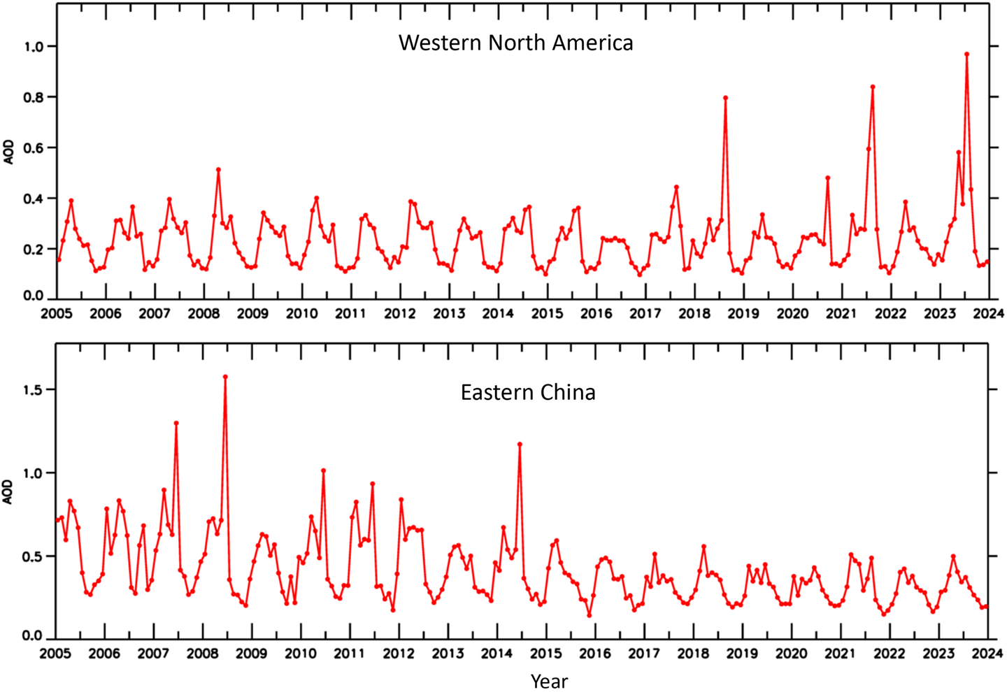
Omar Torres [GSFC] and Changwoo Ahn [GSFC/SSAI] presented regional trend analyses using the re-processed OMI Collection 4 absorbing aerosol product – see Figure 2.

Updates on EOS Synergy Products

Several presenters and posters during the meeting gave updates on EOS synergy products, where OMI data are combined with data from another instrument on one of the EOS flagships. These are described below.

Brad Fisher [SSAI] presented a poster on the Joint OMI–Moderate Resolution Imaging Spectroradiometer (MODIS) cloud products.

Wenhan Qin [GSFC/SSAI] presented a poster on the MODIS–OMI Geometry Dependent Lambertian Equivalent Surface Reflectivity (GLER) product.

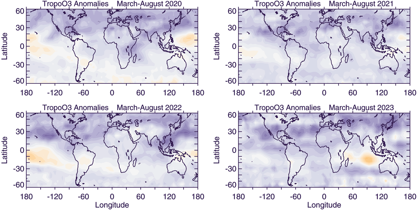
Jerry Ziemke [GSFC and Morgan State University (MSU)] presented on the OMI–MLS Tropospheric Ozone product that showed post-COVID tropospheric O₃ levels measured using this product, which are consistent with similar measurements obtained using other satellite O₃ data – see Figure 3.

Updates on Multisatellite Climate Data Records

The OMI ST also discussed refining and analyzing multisatellite climate data records (CDRs) that have been processed with consistent algorithms. Several presenters reported on this work, who are mentioned below.

Jenny Stavrakou [Koninklijk Belgisch Instituut voor Ruimte-Aeronomie, Royal Belgian Institute for Space Aeronomy (BIRA–IASB)], reported on work focusing on the OMI and TROPOMI HCHO CDR and Huan Yu [BIRA–IASB)] reported harmonized OMI and TROPOMI cloud height datasets based on improved O₂-O₂ absorption retrieval algorithm.

Lok Lamsal [GSFC/UMBC, Goddard Earth Sciences Technology and Research (GESTAR) II], Henk Eskes, and Pepijn Veefkind [KNMI] reported on the OMI and TROPOMI NO₂ CDRs – see Figure 4. 

Si-Wan Kim [Yonsei University, South Korea] reported on OMI and TROPOMI long-term NO₂ trends.

Update on Aura’s Drifting Orbit

Bryan Duncan [GSFC—Aura Project Scientist] closed out the first day with a presentation summarizing predictions of Aura’s drifting orbit. Overall, the impact of Aura’s drift is expected to be minor, and the OMI and MLS teams will be able to maintain science quality data for most data products. He thanked the OMI/TROPOMI ST and user community for expressing their strong support for continuing Aura observations until the end of the Aura mission in mid–2026.

DAY TWO

The second day of the meeting focused on current and upcoming LEO and GEO Atmospheric Composition (AC) missions.

TROPOMI Mission and Data Product Updates

Veefkind presented an update on the TROPOMI mission, which provides continuation and enhancements for all OMI products. Tobias Borssdorf [Stichting Ruimte Onderzoek Nederland (SRON), or Netherlands Institute for Space Research] explained how TROPOMI, with its innovative shortwave infrared (SWIR) spectrometer, measures CH₄ and carbon monoxide (CO). This approach continues measurements that began by the Measurements of Pollution in the Troposphere (MOPITT) instrument on Terra.

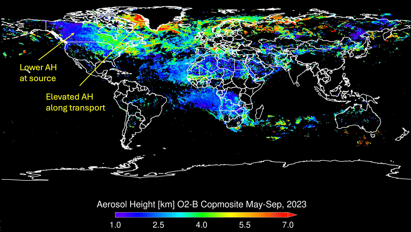
Hiren Jethva [NASA Airborne Science Program] and Torres presented new TROPOMI near-UV aerosol products, including a new aerosol layer optical centroid height product, which takes advantage of the TROPOMI extended spectral range – see Figure 5.

GEMS–TEMPO–Sentinel-4 (UVN): A Geostationary Air Quality Constellation

TROPOMI global observations serve as a de facto calibration standard used to homogenize a new constellation of three missions that will provide AC observations for most of the Northern Hemisphere from GEO. Two of the three constellation members are already in orbit. Jhoon Kim [Yonsei University—PI] discussed the Geostationary Environmental Monitoring Spectrometer (GEMS), launched on February 19, 2020 aboard the Republic of Korea’s GEO-KOMPSAT-2B satellite. It is making GEO AC measurements over Asia. The GEMS team is working on validating measurements of NO₂ diurnal variations using ground-based measurements from the PANDORA Global Network over Asia and aircraft measurements from the ASIA–AQ field campaign.

Liu discussed NASA’s Tropospheric Emission Monitoring of Pollution (TEMPO) spectrometer, launched on April 7, 2023, aboard a commercial INTELSAT 40E satellite. From its GEO vantage point, TEMPO can observe the Continental U.S., Southern Canada, Mexico, and the coastal waters of the Northwestern Atlantic and Northeastern Pacific oceans.

Gonzales Abad [SAO] presented the first measurements from TEMPO. He explained that TEMPO’s design is similar to GEMS, but GEMS includes an additional visible and near infrared (VNIR) spectral channel (540–740 nm) to measure tropospheric O₃, O₂, and water vapor (H₂Ov). TEMPO can perform optimized morning scans, twilight scans, and scans with high temporal resolution (5–10 minutes) over selected regions. Abad reported that the TEMPO team released L1B spectra and the first provisional public L2 products (Version 3), including NO₂, HCHO, and total column O₃. Andrew Rollins [National Oceanic and Atmospheric Administration’s (NOAA) Chemical Sciences Laboratory (CSL)] reported that the TEMPO team is working on validation of provisional data using both ground-based data from PANDORA spectrometers and data collected during several different airborne campaigns completed during the summer of 2023 and compiled on the AGES+ website.

Ben Veihelmann [ESA’s European Space Research and Technology Center—PI] explained that ESA’s Copernicus Sentinel-4 mission will be the final member of the GEO AC constellation. Veefkind summarized the Sentinel-4 mission, which is expected to launch on the Meteosat Third Generation (MTG)-Sounder 1 (MTG-S1) platform in 2025. The mission is dedicated to measuring air quality and O₃ over Europe and parts of the Atlantic and North Africa. Sentinel-4 will deploy the first operational UV-Vis-NIR (UVN) imaging spectrometer on a geostationary satellite. (Airbus will build UVN, with ESA providing guidance.) Sentinel-4 includes two instruments launched in sequence on MTG-S1 and MTG-S2 platforms designed to have a combined lifetime of 15 years. The mission by the European Organisation for the Exploitation of Meteorological Satellites (EUMETSAT) will operate Sentinel-4, and the Deutsches Zentrum für Luft- und Raumfahrt (DLR) or German Aerospace Center will be responsible for operational L2 processing.

These three GEO AC missions, along with the upcoming ESA/EUMETSAT/Copernicus LEO (morning orbit, 9:30 a.m.) Sentinel-5 (S5) mission, will complete a LEO–GEO satellite constellation that will enable monitoring of the most industrialized and polluted regions in the Northern Hemisphere into the 2030s. Sentinel-5 will not continue the OMI–TROPOMI data record in the early afternoon; however, it will be placed in the morning orbit and follow ESA’s Global Ozone Monitoring Experiment (GOME) and EUMETSAT GOME-2 missions. By contrast, GEO AC observations over the Southern Hemisphere are currently not available. Several presenters described ongoing projects for capacity building for LEO satellite air quality data uptake and emission monitoring in Africa and advocated for the new geostationary measurements.

Synergy with Other Current or Upcoming Missions

Attendees discussed the synergy between upcoming AC, GHG, and ocean color missions. Current trends in satellite AC measurements are toward increased spatial resolution and combined observations of short-lived reactive trace gases – which are important for air quality (AQ) monitoring – and long-lived GHG – which are important for climate monitoring and carbon cycle assessments. Some trace gases (e.g., O₃ and CH₄) are both polluters and GHG agents. Others [e.g., NO₂ and sulfur dioxide (SO₂ )] are aerosol [particulate matter (PM)] and O₃ precursors and are used as proxies and spatial indicators for anthropogenic CO₂ and CH₄ emissions.

Yasjka Meijer [ESA—Copernicus Anthropogenic Carbon Dioxide Monitoring (CO₂M) Mission Scientist]) reviewed the plans for CO₂M, which includes high-resolution measurements [~4 km² (~1.5 mi²)] of CO₂ , CH₄ , and NO₂.

Jochen Landgraf [SRON] described ESA’s new Twin Anthropogenic Greenhouse Gas Observers (TANGO) mission, which has the objective to measure CO₂ , CH₄ , and NO₂ at even higher spatial resolution [~300 m (~984 ft)] using two small CubeSat spectrometers flying in formation.

Hiroshi Tanimoto [National Institute for Environmental Studies, Japan] described the Japan Aerospace Exploration Agency’s (JAXA) Global Observing SATellite for greenhouse gases and water cycle (GOSAT-GW) mission, which includes the Total Anthropogenic and Natural Emission mapping SpectrOmeter (TANSO-3) spectrometer to simultaneously measure CO₂ , CH₄, and NO₂ with ~1–3 km (~0.6–1.8 mi) spatial resolution in focus mode. GOSAT-GW will also fly the Advanced Microwave Scanning Radiometer 3 (AMSR3).

Joanna Joiner [GSFC—Geostationary Extended Operations (GeoXO) Project Scientist and ACX Instrument Scientist] described the plans for the next-generation U.S. geosynchronous satellite constellation, which will consist of three satellites covering the full Earth disk: GEO-East, GEO-West, and GEO-Central. (By contrast, the current Geostationary Operational Environmental Satellite (GOES) series has two satellites: GOES–East and GOES–West.) GEO-Central will carry an advanced infrared sounder (GXS) for measuring vertical profiles of many trace gases, temperature and humidity, and a new UV-VIS spectrometer (ACX), which is a follow-on to TEMPO for AQ applications. Both GXS and ACX instruments will be built by BAE Systems, which acquired Ball Aerospace and Technology, and will also build the GeoXO ocean color spectrometer (OCX).

Andrew Sayer [UMBC] described NASA’s Plankton, Aerosols, Clouds, and ocean Ecosystem (PACE), which launched on February 8, 2024. The PACE payload includes a high-spatial resolution [~1 km (~0.6 mi) at nadir] Ocean Color Instrument (OCI), which is a UV-Vis-NIR spectrometer with discrete SWIR bands presenting additional opportunities for synergistic observations with the AC constellation. Sayer presented OCI “first light” aerosol data processed using the unified retrieval algorithm developed by Lorraine Remer [UMBC].

The second day concluded with a joint crossover session with NASA’s Health and Air Quality Applied Sciences Team (HAQAST) followed by a poster session. Several OMI–TROPOMI STM participants presented on a variety of topics that illustrate how OMI and TROPOMI data are being used to support numerous health and AQ applications. Duncan, who is also a member of HAQAST team, presented “20 years of health and air quality applications enabled by OMI data.” He highlighted OMI contributions to AQ and health applications, including NO₂ trend monitoring, inferring trends of co-emitted species [e.g., CO₂, CO, some Volatile Organic Compounds (VOCs)], validation of new satellite missions (e.g., TEMPO, PACE), and burden of disease studies.

DAY THREE

Discussions on the third day focused on advanced retrieval algorithms, leading to new products and new applications for OMI and TROPOMI data. Several presentations described applications of TROPOMI CH₄ data and synergy with small satellites.

Advanced Retrieval Algorithms and New Data Products

Ilse Aben [SRON] described TROPOMI global detection of CH₄ super-emitters using an automated system based on Machine Learning (ML) techniques – see Figure 6. Berend Schuit [SRON] provided additional detail on these methods. He introduced the TROPOMI CH₄ web site to the meeting participants. He explained how TROPOMI global CH₄ measurements use “tip-and-cue” dedicated satellites with much higher spatial resolution instruments [e.g., GHGSat with ~25-m (~82-ft) resolution] to scan for individual sources and estimate emission rates. Most CH₄ super-emitters are related to urban areas and/or landfills, followed by plumes from gas and oil industries and coal mines.

Alba Lorente [Environmental Defense Fund—Methane Scientist] introduced a new MethaneSAT satellite launched in March 2024, which aims to fill the gap in understanding CH₄ emissions on a regional scale [200 x 200 km² (~77 x 77 mi²)] from at least 80% of global oil and gas production, agriculture, and urban regions. Alex Bradley [University of Colorado, Boulder] described improvements to TROPOMI CH₄ retrievals that were achieved by correcting seasonal effects of changing surface albedo.

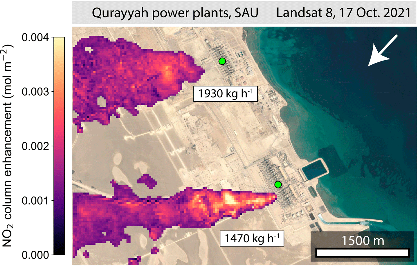
Daniel Jacob [Harvard University] presented several topics, including the highest resolution [~30 m (~98 ft)] NO₂ plume retrievals from Landsat-8 – see Figure 7 – and Sentinel-2 imagers. He also discussed using a ML technique trained with TROPOMI data to improve NO₂ retrievals from GEMS and modeling NO₂ diurnal cycle and emission estimates. He introduced the ratio of ammonia (NH₃) to NO₂ (NH₃/NO₂) as an indicator of particulate matter with diameters less than 2.5 µm (PM_2.5) nitrate sensitivity regime. Jacob emphasized the challenges related to satellite NO₂ retrievals (e.g., accounting for a free-tropospheric NO₂ background and aerosols).

Steffen Beirle [Max Planck Institute for Chemistry, Germany] explained his work to fit TROPOMI NO₂ column measurements to investigate nitric oxide (NO) to NO₂ processing in power plant plumes. Debra Griffin [Environment and Climate Change Canada (ECCC)] used TROPOMI NO₂ observations and ML random forest technique to estimate NO₂ surface concentrations. Sara Martinez-Alonso [NCAR] investigated geographical and seasonal variations in NO₂ diurnal cycle using GEMS and TEMPO data.  Ziemkecombined satellite O₃ data to confirm a persistent low anomaly (~5–15%) in tropospheric O₃ after 2020.  Jethva presented advanced OMI and TROPOMI absorbing aerosol products. Yu described improved OMI and TROPOMI cloud datasets using the O₂-O₂ absorption band at 477 nm. Nicholas Parazoo [Jet Propulsion Laboratory (JPL)] described TROPOMI Fraunhofer line retrievals of red solar-induced chlorophyll fluorescence (SIF) near O₂-B band (663–685 nm) to improve mapping of ocean primary productivity. Liyin He [Duke University] described using satellite terrestrial SIF data to study the effect of particulate pollution on ecosystem productivity.

New Applications

Zachary Fasnacht [SSAI] used OMI and TROPOMI spectra to train a neural network to gap-fill MODIS and Visible Infrared Imaging Radiometer Suite (VIIRS) ocean color data under aerosol, sun glint, and partly cloudy conditions. This ML method can also be applied to PACE OCI spectra. Anu-Maija Sundström [Finnish Meteorological Institute (FMI)] used OMI and TROPOMI SO₂ and O₃ data as proxies to study new particle formation events. Lindsey Anderson [University of Colorado, Boulder] described how she used TROPOMI NO₂ and CO measurements to estimate the composition of wildfire emissions and their effect on forecasted air quality. Heesung Chong [SAO] applied OMI bromine oxide (BrO) retrievals to the NOAA operational Ozone Mapping and Profiling Suite Nadir Mapper (OMPS-NM) on joint NOAA–NASA Suomi-National Polar-orbiting Partnership (Suomi NPP) satellite with the possibility to continue afternoon measurements using similar OMPS-NM instruments on the four Joint Polar Satellite System missions (JPSS-1,-2,-3,-4) into the 2030s. (JPSS-1 and -2 are now in orbit and known as NOAA-20 and -21 respectively; JPSS-4 is planned for launch in 2027, with JPSS-3 currently targeted for 2032.)

Kim demonstrated the potential for using satellite NO₂ and SO₂ emissions as a window into socioeconomic issues that are not apparent by other methods. For example, she showed how OMI and TROPOMI data were widely used to monitor air quality improvements in the aftermath of COVID-19 lockdowns. (Brad Fisher [SSAI] presented a poster on a similar topic.)

Cathy Clerbaux [Center National d’Études Spatiale (CNES), or French Space Agency] showed how her team used TROPOMI NO₂ data to trace the signal emitted by ships and used this information to determine how the shipping lanes through the Suez Canal changed in response to unrest in the Middle East. Iolanda Ialongo [FMI] showed a similar drop of NO₂ emissions over Donetsk region due to the war in Ukraine. Levelt showed how OMI and TROPOMI NO₂ data are used for capacity-building projects and for air quality reporting in Africa. She also advocated for additional geostationary AQ measurements over Africa.

DAY FOUR

Discussions on the final day focused on various methods of assimilating satellite data into air quality models for emission inversions and aircraft TEMPO validation campaigns. The meeting ended with Levelt giving her unique perspective on the OMI mission, as she reflected on more than two decades being involved with the development, launch, operation, and maintenance of OMI.  

Assimilating Satellite Data into Models for Emissions

Brian McDonald [CSL] described advance chemical data assimilation of satellite data for emission inversions and the GReenhouse gas And Air Pollutants Emissions System (GRA²PES). He showed examples of assimilations using TROPOMI and TEMPO NO₂ observations to adjust a priori emissions. He also showed that when TEMPO data are assimilated, NO_x emissions adjust faster and tend to perform better at the urban scale. Adrian Jost [Max Planck Institute for Chemistry] described the ESA-funded World Emission project to improve pollutant and GHG emission inventories using satellite data. He showed examples of TROPOMI SO₂ emissions from large-point sources and compared the data with bottom-up and NASA SO₂ emissions catalogue.

Ivar van der Velde [SRON] presented a method to evaluate fire emissions using new satellite imagery of burned area and TROPOMI CO. Helene Peiro [SRON] described her work to combine TROPOMI CO and burned area information to compare the impact of prescribed fires versus wildfires on air quality in the U.S. She concluded that prescribed burning reduces CO pollution. Barbara Dix [University of Colorado, Boulder, Cooperative Institute for Research in Environmental Sciences] derived NO_x emissions from U.S. oil and natural gas production using TROPOMI NO₂ data and flux divergence method. She estimated TROPOMI CH₄ emissions from Denver–Julesburg oil and natural gas production. Dix explained that the remaining challenge is to separate oil and gas emissions from other co-located CH₄ sources. Ben Gaubert [NCAR, Atmospheric Chemistry Observations and Modeling] described nonlinear and non-Gaussian ensemble assimilation of MOPITT CO using the data assimilation research testbed (DART).

Andrew (Drew) Rollings [CSL] presented first TEMPO validation results from airborne field campaigns in 2023 (AGES+ ), including NOAA CSL Atmospheric Emissions and Reactions observed from Megacities to Marine Aeras (AEROMMA) and NASA’s Synergistic TEMPO Air Quality Science (STAQS) campaigns.

A Reflection on Twenty Years of OMI Observations

Levelt gave a closing presentation in which she reflected on her first involvement with the OMI mission as a young scientist back in 1998. This led to a collaboration with the international ST to develop the instrument, which was included as part of Aura’s payload when it launched in July 2004. She reminisced about important highlights from 2 decades of OMI, e.g., the 10-year anniversary STM at KNMI in 2014 (see “Celebrating Ten Years of OMI Observations,” The Earth Observer, May–Jun 2014, 26:3, 23–30), and the OMI ST receiving the NASA/U.S. Geological Survey Pecora award in 2018 and the American Meteorological Society’s Special award in 2021.

Levelt pointed out that in this combined OMI–TROPOMI meeting the movement towards using air pollution and GHG data together became apparent. She ended by saying that the OMI instrument continues to “age gracefully” and its legacy continues with the TROPOMI and LEO–GEO atmospheric composition constellation of satellites that were discussed during the meeting.

Conclusion

Overall, the second OMI–TROPOMI STM acknowledged OMI’s pioneering role and TROPOMI’s unique enhancements in measurements of atmospheric composition: 

1. Ozone Layer Monitoring: Over the past two decades, OMI has provided invaluable data on the concentration and distribution of O₃ in the Earth’s stratosphere. This data has been crucial for understanding and monitoring the recovery of the O₃ layer following international agreements, such as the Montreal Protocol.
2. Air Quality Assessment: OMI’s high-resolution measurements of air pollutants, such as NO₂, SO₂, and HCHO, have significantly advanced our understanding of air quality. This information has been vital for tracking pollution sources, studying their transport and transformation, and assessing their impact on human health and the environment.
3. Climate Research: The data collected by OMI has enhanced our knowledge of the interactions between atmospheric chemistry and climate change. These insights have been instrumental in refining climate models and improving our predictions of future climate scenarios.
4. Global Impact: The OMI instrument has provided near-daily global coverage of atmospheric data, which has been essential for scientists and policymakers worldwide. The comprehensive and reliable data from OMI has supported countless research projects and informed decisions aimed at protecting and improving our environment.

OMI remains one of the most stable UV/Vis instruments over its two decades of science and trend quality data collection. The success of the OMI and TROPOMI instruments is a testament to the collaboration, expertise, and dedication of both teams.

Nickolay Krotkov
NASA’s Goddard Space Flight Center
Nickolay.a.krotkov@nasa.gov

Pieternel Levelt
National Center for Atmospheric Research, Atmospheric Chemistry Observations & Modeling
levelt@ucar.edu

Powered by WPeMatico

Get The Details…

Artemis II Orion Spacecraft Undergoes Testing

Teams lifted NASA’s Orion spacecraft for the Artemis II test flight out of the Final Assembly and System Testing cell and moved it to the altitude chamber to complete further testing on Nov. 6 inside the Neil A. Armstrong Operations and Checkout building at NASA’s Kennedy Space Center in Florida.

Engineers returned the spacecraft to the altitude chamber, which simulates deep space vacuum conditions, to complete the remaining test requirements and provide additional data to augment data gained during testing earlier this summer.

The Artemis II test flight will be NASA’s first mission with crew under the Artemis campaign, sending NASA astronauts Victor Glover, Christina Koch, and Reid Wiseman, as well as CSA (Canadian Space Agency) astronaut Jeremy Hansen, on a 10-day journey around the Moon and back.

Image credit: Lockheed Martin/David Wellendorf

Powered by WPeMatico

Get The Details…
Elyna Niles-Carnes

Station Science Top News: Nov. 8, 2024

Researchers demonstrated the feasibility of 3D bioprinting a meniscus or knee cartilage tissue in microgravity. This successful result advances technology for bioprinting tissue to treat musculoskeletal injuries on long-term spaceflight or in extraterrestrial settings where resources and supply capacities are limited.

BFF Meniscus-2 evaluated using the BioFabrication Facility to 3D print knee cartilage tissue using bioinks and cells. The meniscus is the first engineered tissue of an anatomically relevant shape printed on the station. Manufactured human tissues have potential as alternatives to donor organs, which are in short supply. Bioprinting in microgravity overcomes some of the challenges present in Earth’s gravity, such as deformation or collapse of tissue structures.

Complex cultures of central nervous system cells known as brain organoids can be maintained in microgravity for long periods of time and show faster development of neurons than cultures on Earth. These findings could help researchers develop treatments for neurodegenerative diseases on Earth and address potential adverse neurological effects of spaceflight.

Cosmic Brain Organoids examined growth and gene expression in 3D organoids created with neural stem cells from individuals with primary progressive multiple sclerosis and Parkinson’s disease. Results could improve understanding of these neurological diseases and support development of new treatments. Researchers plan additional studies on the underlying causes of the accelerated neuron maturation.

Researchers demonstrated that induced pluripotent stem cells (iPSCs) can be processed in microgravity using off the-shelf cell culture materials. Using standard laboratory equipment and protocols could reduce costs and make space-based biomedical research accessible to a broader range of scientists and institutions.

Stellar Stem Cells Ax-2 evaluated how microgravity affects methods used to generate and grow stem cells into a variety of tissue types on the ground. iPSCs can give rise to any type of cell or tissue in the human body, and insight into processing in space could support their use in regenerative medicine and future large-scale biomanufacturing of cellular therapeutics in space.

Powered by WPeMatico

Get The Details…
Sumer Loggins