Tracking Glacial Change with Landsat and Radar 

Tracking Glacial Change with Landsat and Radar 

An animation shows glaciers in the Karakoram range of Pakistan with monthly ice-velocity measurements overlaid from January through December. On Baltoro Glacier, red areas, indicating high ice velocities, propagate slowly downslope throughout the melting season.
NASA/Chad Greene

For the first time, scientists have created a comprehensive global dataset revealing how the world’s glaciers speed up and slow down with the seasons. Published in Science in November 2025, this groundbreaking study analyzed over 36 million satellite image pairs—including decades of Landsat data—to track the seasonal “pulse” of every major glacier on Earth.

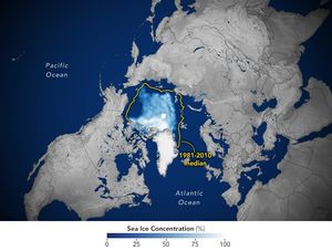
The research, built off the ITS_LIVE ice velocity dataset from NASA’s Jet Propulsion Laboratory (JPL), reveals that seasonal glacier dynamics are becoming more pronounced as our planet warms, with the strongest seasonal variations occurring where annual maximum temperatures exceed freezing. Armed with this global perspective, researchers can continue to tease out patterns in glacial dynamics, identifying how factors including geology and hydrology impact seasonal melting. 

Alex Gardner, a scientist at NASA JPL and a co-author on this study, explains how combining Landsat and radar data makes this research possible.

What makes this research unique from other studies of glacial dynamics? 

While many past studies have investigated seasonal changes in glacier flow, they have typically focused on single glaciers or specific regions. This localization makes it difficult to extrapolate findings to the rest of the world.

This study is the first to characterize seasonal flow changes for all the world’s glaciers. By applying a consistent methodology globally, we were able to isolate the universal relationships that drive seasonal fluctuations in glacier flow.

Why did you use Landsat in this work? Did it give you any insight that would have been difficult to get otherwise?

We utilized data from Landsat 4/5/7/8/9, as well as ESA’s Sentinel 2 (optical) and Sentinel 1 (radar). Landsat offers an unmatched historical record with dense temporal sampling, particularly following the launch of Landsat 8 in 2013.

Three factors make Landsat imagery ideal for detecting “surface displacements” (the subtle pixel shifts used to estimate flow):

  • Near-exact repeat orbits: The satellite returns to the exact same position.
  • Nadir viewing: The instrument looks directly downward.
  • Stable instrument geometry: Distortion is minimized.
An animation shows glaciers in southeastern Alaska with monthly ice-velocity measurements overlaid from January through December. Red areas, indicating high ice velocities, begin to expand across Malaspina Glacier in spring.
NASA/Chad Greene

Why does the ITS_LIVE tool use the Landsat panchromatic band? Which bands from Landsats 4-5 are used?

We measure surface displacement using a technique called feature tracking, which tracks the movement of specific surface details between a primary and a secondary image.

This approach works best with high-resolution imagery because there are more “features” to track. Therefore, we utilize the 15m panchromatic band. For the older Landsat 4/5 data, we use Band 2 (visible red) because it provides the best contrast over bright glacier surfaces.

You used Landsat data in combination with radar data to track ice velocity. What did each of these datasets contribute? 

Optical and Radar imagery are highly complementary and allow us to reconstruct a complete timeline of glacier flow:

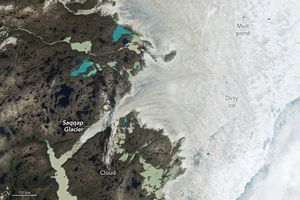
  • Radar (Active Sensor): Can image the surface day or night, regardless of cloud cover, but struggles with feature tracking when the surface is melting (wet snow/ice).
  • Optical (Passive Sensor): Requires sunlight and clear skies, but performs significantly better than radar when the surface is melting.

How did you use radar data to validate uncertainties? 

We characterized uncertainty by analyzing retrieved velocities over stationary surfaces, such as bedrock. If our data showed high variability or movement in areas we know are not moving (like rock), we knew those measurements carried a higher uncertainty.

You found that glacier dynamics vary by region and glacier type. Why is it important to understand these global differences? 

A glacier’s response to external forces—such as meltwater lubricating the bedrock or changes in frontal melting—is highly dependent on local factors (e.g., the material beneath the glacier or the shape of the fjord). This makes it risky to assume that findings from one glacier apply to another.

Our study identified general patterns by observing nearly every glacier on Earth. A key finding was the relationship between temperature and flow:

Seasonal variability becomes prominent when annual maximum temperatures exceed 0°C.

The amplitude of that seasonal cycle increases with every degree of warming above that threshold.

Are there plans to incorporate Landsat 9 data into future studies? How would improvements in remote sensing technology (increased temporal revisit, spatial resolution, etc.) impact glacial velocity analyses?

We are already ingesting Landsat 9 data into the ITS_LIVE project, which is designed to scale quickly with new sensors. Future sensor improvements offer a trade-off:

  • Increased Spatial Resolution: Allows us to track a higher number of surface features, improving flow estimates.
  • Increased Temporal Frequency: Reduces data gaps caused by surface changes (loss of features), but can potentially increase error rates. This is because displacement is an accumulated signal; features move half the distance in an 8-day pair compared to a 16-day pair, making the movement harder to distinguish from background noise.

Are there any research questions you’re interested in that build off this work?

This study is just the tip of the iceberg. The dataset is rich with insights on glacier mechanics that are waiting to be uncovered. While we hope to make new discoveries in the coming years, we are equally excited to see what breakthroughs come from the wider scientific community exploring this open data.

An animation shows an ice cap in the Canadian Arctic with monthly ice-velocity measurements overlaid from January through December. Red areas, indicating high ice velocities, expand across the ice cap during the summer months.
NASA/Chad Greene

Explore More

Tracking Glacial Change with Landsat and Radar 

5 min read

NASA Scientist Alex Gardner highlights how Landsat made his research into the dynamics of glacial flow possible.

Feb 4, 2026
Article

Chilled New York City

3 min read

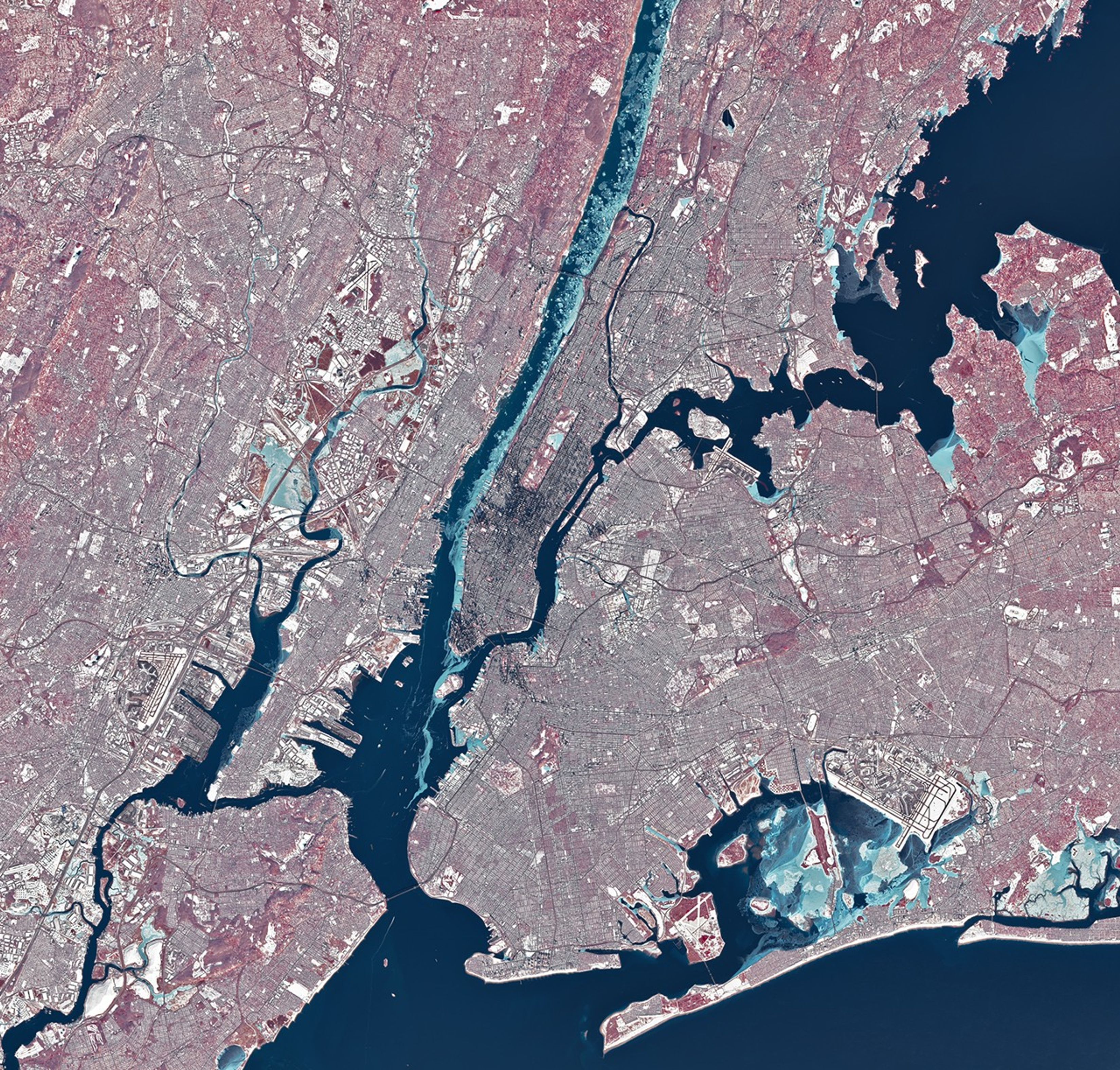
Ice in the Hudson River hugged the shore of Manhattan amid a deep freeze.

Feb 4, 2026
Article

Cracking Antarctic Sea Ice

4 min read

Icebreakers play a critical role in delivering supplies to America’s largest research base in Antarctica.

Feb 3, 2026
Article

Powered by WPeMatico

Get The Details…

Chilled New York City

Chilled New York City

Chunks of ice, which appear light blue in this false-color image, line the western shore of Manhattan in the Hudson River. Smaller rivers and lakes in the scene also appear frozen or partially frozen. The ground is snow-covered, and tall buildings cast long, dark shadows.
January 28, 2026

The New York metropolitan area was showing the effects of a prolonged cold spell in late January 2026. During a stretch of frigid weather, ice choked the Hudson River along Manhattan’s western shore.

The OLI (Operational Land Imager) on Landsat 8 captured this image of the wintry landscape around midday on January 28. The image is false-color (bands 5-4-3) to distinguish ice (light blue) from open water and snow. Vegetation appears red. Ice is abundant in the Hudson River and visible in smaller amounts in the East River, the Jacqueline Kennedy Onassis Reservoir in Central Park, and waterways in New Jersey.

Temperatures in New York City dropped below freezing on January 24 and stayed there for over a week. The high on January 28, the date of the image, was 23 degrees Fahrenheit (minus 5 degrees Celsius). Low temperatures and harsh wind chills gripped much of eastern North America over this period amid a surge of Arctic air.

Much of the ice in the image likely floated there from farther upriver, where tidal currents are weaker and salinity is lower. These conditions allow water to freeze sooner and at higher temperatures than the faster-flowing, brackish water near the river’s mouth, shown here. A complete freeze of the Hudson around Manhattan is unlikely, experts say, although it did occur back in 1888. Still, the ice buildup was substantial enough for NYC Ferry to suspend services for several days.

Iced-up rivers can have other implications, from flooding and infrastructure damage to changes in hydrologic processes that affect water quality and aquatic habitats.

Scientists, government agencies, and emergency responders are increasingly turning to remote sensing technologies such as synthetic aperture radar and hyperspectral imaging to track river ice. Improved monitoring can aid in water resource management and mitigate ice’s effects on infrastructure and ecosystems.

In addition to the river ice, other signs of winter were visible across New York. A fresh layer of snow coated the landscape following a winter storm, in which a weather station in Central Park recorded nearly 12 inches (30 centimeters) of accumulation on January 25. And the low angle of the midwinter Sun caused the tall buildings in Midtown and Lower Manhattan to cast long shadows.

In a neighboring borough on February 2, a shorter shadow was cast—this one by the weather-prognosticating groundhog known as Staten Island Chuck. Folklore holds that the sighting signals six more weeks of winter. When compared with data from NOAA’s National Centers for Environmental Information, the New York rodent was deemed the most accurate of his peer weather “forecasters.” This year, Chuck might be right, at least in the near term: the National Weather Service forecast called for below-average temperatures to persist, with Arctic air returning to the city by the weekend.

NASA Earth Observatory image by Michala Garrison, using Landsat data from the U.S. Geological Survey. Story by Lindsey Doermann.

References & Resources

You may also be interested in:

Stay up-to-date with the latest content from NASA as we explore the universe and discover more about our home planet.

Arctic Sea Ice Ties for 10th-Lowest on Record

3 min read

Satellite data show that Arctic sea ice likely reached its annual minimum extent on September 10, 2025.

Article

Greenland Ice Sheet Gets a Refresh

3 min read

A moderately intense season of surface melting left part of the ice sheet dirty gray in summer 2025, but snowfall…

Article

Antarctic Sea Ice Saw Its Third-Lowest Maximum

2 min read

Sea ice around the southernmost continent hit one of its lowest seasonal highs since the start of the satellite record.

Article

Powered by WPeMatico

Get The Details…

Biomedical Research, CubeSat Deployments Top Crew Schedule

Biomedical Research, CubeSat Deployments Top Crew Schedule

This tranquil view from the International Space Station captures the Kibo laboratory module with its Exposed Facility, a portion of the station’s main solar arrays (right), and part of the Canadarm2 robotic arm (left). The photograph was taken during an orbital sunset as the station soared 270 miles above a cloudy Atlantic Ocean off the coast of South Africa.
This tranquil view from the International Space Station captures the Kibo laboratory module with its Exposed Facility, a portion of the station’s main solar arrays (right), and part of the Canadarm2 robotic arm (left) above a cloudy Atlantic Ocean.
NASA

Biomedical research to keep crews healthy and CubeSat deployments for educational research topped the science schedule aboard the International Space Station on Tuesday. The Expedition 74 crew also focused on cargo swaps and life support maintenance throughout the day.

NASA Flight Engineer Chris Williams processed his body samples during the first half of his shift for the long-running CIPHER astronaut health study. He collected then stowed his urine samples inside a science freezer for preservation and later analysis. The human research investigation looks at a broad range of physiological and psychological parameters before, during, and after a spaceflight to understand how the human body adapts to weightlessness. Doctors will use the insights to keep crews healthy as they travel farther away from Earth.

Williams also pointed a camera out a window on the cupola as a set of CubeSats were deployed outside the Kibo laboratory module by a small satellite orbital deployer into Earth orbit. Students from Mexico, Italy, Thailand, Malaysia, and Japan designed the shoe-boxed satellites for a series of Earth observations and technology demonstrations.

Williams also logged onto a station computer and studied procedures to monitor the approach and rendezvous of the SpaceX Crew-12 mission aboard a Dragon spacecraft targeted to launch no earlier than Feb. 11 from Cape Canaveral in Florida. The first-time space flyer then continued packing completed science experiments and station hardware for return to Earth inside a Dragon spacecraft docked to the Harmony module’s forward port.

Flight Engineer Sergei Mikaev started his shift in the Nauka science module replacing battery controllers to maintain safe operations of the Roscosmos segment’s electrical power system. After lunchtime, Mikaev inspected and cleaned a pair of laptop computers before removing hardware and crew supplies from the Progress 92 cargo craft and stowing them inside the orbital outpost.

Station Commander Sergey Kud-Sverchkov spent his shift primarily on lab maintenance in the station’s Roscosmos’ modules. He first verified the location and configuration of a variety tool kits then inventoried and photographed the tools for analysis on the ground. Afterward, Kud-Sverchkov cleaned and inspected station smoked detectors and their components verifying they were in functional condition.

Learn more about station activities by following the space station blog, @space_station on X, as well as the ISS Facebook and ISS Instagram accounts.

Get the latest from NASA delivered every week. Subscribe here.

Powered by WPeMatico

Get The Details…

Mark A. Garcia

Full Moon over Artemis II

Full Moon over Artemis II

A golden full moon is seen shining over NASA’s SLS (Space Launch System) and Orion spacecraft, atop the mobile launcher in the early hours of February 1, 2026. The SLS core stage is a distinctive deep orange, while Orion is white and sits on top of the core stage.
NASA/Sam Lott

A full moon is seen shining over NASA’s SLS (Space Launch System) and Orion spacecraft, atop the mobile launcher at Launch Pad 39B at NASA’s Kennedy Space Center in Florida in the early hours of February 1, 2026.

The agency concluded a wet dress rehearsal for the agency’s Artemis II test flight early Tuesday morning, successfully loading cryogenic propellant into the SLS (Space Launch System) tanks, sending a team out to the launch pad to closeout Orion, and safely draining the rocket. The wet dress rehearsal was a prelaunch test to fuel the rocket, designed to identify any issues and resolve them before attempting a launch. To allow teams to review data and conduct a second wet dress rehearsal, NASA now will target March as the earliest possible launch opportunity for the flight test.

Read more about the wet dress rehearsal.

Image credit: NASA/Sam Lott

Powered by WPeMatico

Get The Details…
Monika Luabeya

NASA Space to Soil Challenge

NASA Space to Soil Challenge

A 3D rendering of a satellite with solar panels and a wire mesh antenna orbiting Earth. The Earth is textured with continents and oceans. The satellite is in the foreground against a dark background with stars.
NASA/JPL-Caltech

Rapid advances in commercial space, artificial intelligence, and edge computing are transforming what is possible for Earth observation. By pushing more intelligence onboard, missions can move from passively collecting data to actively interpreting and responding to changing surface conditions in near-real time, enabling more targeted observations and dramatically improving the value of data returned to the ground. Within this context, land-focused applications such as regenerative agriculture, sustainable forestry, and broader land resilience efforts stand to benefit enormously from satellites that can adapt what, when, and how they sense based on dynamic environmental signals and algorithmic insight rather than fixed schedules or static acquisition plans.

NASA Earth Science Technology Office (ESTO) invites participants to design small satellite (SmallSat) mission concepts that leverage adaptive sensing and onboard processing to enhance regenerative agriculture, forestry, or a similar land resilience objective.​ Participants must work within onboard power, compute, and bandwidth constraints characteristic of SmallSat missions, focusing on how to orchestrate existing land observation algorithms into an efficient, responsive onboard intelligence layer.​ Both hardware-oriented and software-oriented solutions—or combinations of the two—are encouraged.

NASA’s primary objective for this challenge is to advance computational and systems approaches for adaptive sensing or onboard processing on SmallSat missions. The goal is not to develop new agricultural or forestry science but rather to improve how SmallSats sense, process, and deliver information to enable these applications.

Award: $400,000 in total prizes

Challenge Open Date: January 30, 2026

Submission Close Date: May 4, 2026

For more information, visit: https://nasa-space-to-soil.org/

Powered by WPeMatico

Get The Details…
Bailey G. Light